Introduction
In this blog, we are going to tell about the IAM [1] paper and how we tried to reproduce some results of that paper. The title of the IAM paper is Influence-aware memory architectures for deep reinforcement learning and authored by Miguel Suau et al. The idea of the project was to reimplement the IAM model with a different library and to reproduce some results given in the paper. The main idea the paper proposes is an architecture where the agent has some influence-aware memory (IAM). The agent makes its decisions based on a reinforcement learning model. With this architecture, it is then possible to remember the useful information from the environment while alleviating the training difficulties compare to conventional methods using RNNs. The goal of the paper is to show that architecture indeed has an important effect on convergence, learning speed and performance of the agent. We reproduced the implementation and repeated some of the experiments described in the paper to see if we got some similar results.
The design of the IAM described will be explained in greater detail in the next section. After that, we will dive into our implementation and the results we got from that implementation. At last, we discuss our results in a comparison with that of the paper and give a short conclusion of the project.
The design of IAM
As introduced in the introduction the IAM stands for influence aware memory, meaning that the architecture is intended to only remember relevant parts of the environment. This is done by letting the RNN focus on a fraction of the environment or observations.
The model is used with an agent that uses reinforcement learning (RL). In reinforcement learning, the main characters are the agent and the environment. The environment is the place where the agent makes observations and with which it interacts. Each iteration the agent sees an observation of the state of the environment, based on these observations the agent makes decisions out of a certain set of possible actions. This way the agent moves or interacts with its environment and get its rewards. This reward tells the agent how good it is performing. The goal of reinforcement learning is to get an agent that gives a high reward i.e. performs well.
The actual RL algorithm which is used to train the model is the Proximal Policy Optimization (PPO) [2]. This algorithm focuses on taking the biggest steps possible to improve, without stepping so far that the performance suddenly collapses.
Now having explained the RL part of the system let’s discuss the IAM architecture. This model consists of two main parts, the FNN and an RNN. These two parts are used in parallel, as can be seen in Figure 1. The FNN lets all information flow and the RNN is the memory part of the model, together they form the decision of the agent. The RNN is implemented as an LSTM [3]. Because memorizing all observed variables can be costly or requires unnecessary effort, the RNN is restricted on the information it can memorize. This restriction can be either done by reducing the size of the RNN itself or reducing the observation it receives.
The paper describes the use of a d-set to reduce the observation information. This set is the information that is relevant to be remembered. The selection operator D which determines the d-set, depicted in Figure 1, can be a manual set or learned. For environments where the designer can guess the variables which influence the hidden state, the manual option is a viable choice. However for more complex environments, one wants to learn this selection operator. There are two different versions here. The static set and dynamic one. The static set can be used in environments where the interesting parts of the environment do not change over time, while dynamic can be used when they do. For example, when playing pong the ball and players move constantly in the environment. The direction of the ball is relevant to remember, a dynamic selection operator is needed to select the area where the ball is.
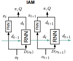 Diagram of the IAM model from Figure 3 of the paper.
With this design, the IAM model aims at good convergence, learning speed and performance of the agent
Implementation in Pytorch
The IAM model for the Warehouse environment is relatively simple to create. However, some information in the paper is missing which took more time to figure out. In short, we have taken these steps to reproduce the paper: Selecting a similar PPO algorithm, adapting the Warehouse environment to work with OpenAI Gym and combine a FNN with GRU in parallel to create the IAM model.
Our parameters should be the same as in the paper following the default PPO settings. However, after generating all the results we found out that the paper uses a ppo epoch of 3 and our implementation 4. This can affect the output, but we are not comparing the absolute results, only the relative results to the baselines so this is less of a problem. Also, our GRU model does not have an FNN as first layer which would have been better for comparison in hindsight.
PPO algorithm
The author implemented his own PPO algorithm, we choose to use an algorithm based on OpenAi PPO from this repo. The code already had some structure for a recurrent network namely the GRU, this why we created our IAM with a GRU instead of an LSTM. Using the GRU will change the results compared to the paper, but we can still relate the performance of the IAM model to a single GRU.
Warehouse
The Warehouse environment is created by the author himself. It contains one agent in a 7x7 grid which needs to collect items at boundaries of the grid to receive a reward. These items appear at random and disappear after 8 seconds, so the model needs some kind of memory to save this information for multiple timesteps.
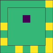
Warehouse visualization. (blue) agent, (yellow) items.
Fortunately, the code is available on Github, and so we could easily copy the environment. The environment is also clearly explained in the paper, so we could have created it ourselves.
Two small adjustments have been made to get the environment working with the PPO algorithm:
- The observation space property with the correct output was added
- Metadata property set to None
IAM model
As described in the paper the basic IAM model for the Warehouse environment uses an FNN and GRU in parallel. The paper didn’t explain how the IAM model was used in the PPO algorithm. This is an important detail since the algorithm uses an actor and critic model, and these can be used in different combinations. For example parts of the model used in the actor and critic can be shared or completely separate. We decided to use two instances of the IAM model, one as actor and one as critic.
D-set
We looked at how to implement the d-set functionality of the model. We did this by reducing the size of the RNN to one layer of 25 parameters. This increased the training speed. But we saw no real increase in performance. As the d-set mainly impacts dynamic environments we left this out of the model we used in our experiments.
Baselines
Since we use a different PPO model as the original paper, to compare the results correctly, the baselines used in the paper are also implemented, again using two instances of the model for actor and critic:
- A single FNN of two layers with one or eight observations as input. With hidden sizes to be the same as in the paper: 640,256.
- A single GRU. Containing just one layer of 128 parameters.
Results
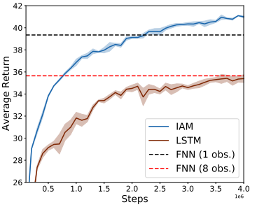
With the experiments, we mainly focused on reproducing Figure 5 of the paper . In this figure, we can see the training graphs of different models. As explained in the design section the paper uses LSTM in the IAM this is also what it is compared against. The other two horizontal lines are the FNN’s with different setting for the observations. We chose this graph because is it gave a clear comparison between the proposed model plus others and because it used the warehouse environment, for which we also had a good working implementation.
Below we have two figures that are the results of the reproduced implementation. The first one is with a minibatch of 8 and the other one with 32. The figure of the paper also uses a minibatch of 32. As explained in the implementation section we used GRU as the RNN implementation, so we also compare this to the IAM.
The experiments were done on a laptop and google cloud server both using linux. Using among other things the torch threads we could run multiple processes, up to 32. The FNN 1,8 and GRU took on average less or around 4 hours, while the IAM took 5 hours on average.
In the first figure, we notice that the FNN with one observation gives the best result and the FNN 8 the worse. In the second figure, both FNNs give the lowest returns. More interesting is the GRU IAM comparision. We see in both figures that the GRU is doing an overall better job than the IAM model. This is a different result than the paper presents. The paper claimed that the GRU and LSTM are less stable. But if we look at the variance of the GRU in our figures this is not greater than the IAM model.
The final returns and runtimes are also summed up in the table.
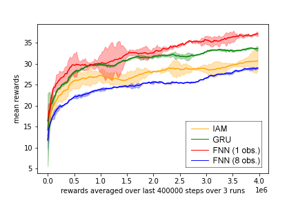 Minibatch of 8 with four different models
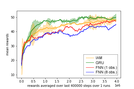 Minibatch of 32 with four different models
| Model | Minibatch | Average runtime | Return |
|---|---|---|---|
| GRU | 8 | 4 hours | 33.6 |
| IAM | 8 | 5 hours | 30,7 |
| FNN 1 | 8 | 2 hours 11 min | 37 |
| FNN 8 | 8 | 3 hours 49 min | 28,9 |
| GRU | 32 | 3 hours 49 min | 49,9 |
| IAM | 32 | 4 hours 51 min | 48,2 |
| FNN 1 | 32 | 3 hours 30 min | 47,3 |
| FNN 8 | 32 | 4 hours 15 min | 45 |
Reproducibility
Overall, the information from the paper was sufficient to implement the model described.
But as also discussed earlier the paper does miss some important details.
When creating the plots of our result and comparing it to Figure 5 of the paper, we noticed that information was missing on how the graphs were created in the paper.
These are the scale of the reward (can be guessed to be multiplied by 100),
the amount of timesteps used in the rolling average and
how many training runs have been used to find the variation. Luckily, the author replied quickly to our emails to give this additional information and this adds to the reproducibility factor as is mentioned here [4].
Also, some other inconsistencies were found in the paper and appendix reducing the reproducibility.
- The observations used in the FNN were different in the paper (8) and the appendix (32).
- The size of each model should be equal according to the appendix but that LSTM is described to have 128 less neurons.
- We were also not sure what to do with the time horizon parameter as it isn’t explained anywhere in the paper.
Conclusion
The reproducibility of the paper was good. Some information was missing, but the author quickly responded to any of our questions. We did however see different results than the author was claiming. The IAM network containing the FNN and GRU did not have a higher performance than just a single GRU. On average the GRU performed slightly better, and the training time was also 20% faster compared to the IAM network. Our intuition tells us that this is because the GRU model has much fewer parameters than the IAM network. In hindsight, after all the results had been created, it would have been better to have the same number of parameters for each model for a better comparison. This is also mentioned in the paper.
We do want to note that we did not do any experiments with the Atari environments because of the long training time and the author does claim that the advantage of the IAM model becomes more apparent when increasing the dimensionality of the problem. That’s, for future work.
Links
Authors implementation: https://github.com/INFLUENCEorg/influence-aware-memory
Paper: https://arxiv.org/pdf/1911.07643.pdf
PPO implementation used: https://github.com/ikostrikov/pytorch-a2c-ppo-acktr-gail
References
[1]
Suau, M., Congeduti, E., Starre, R., Czechowski, A., & Oliehoek, F. A. (2019). Influence-aware memory for deep reinforcement learning. arXiv preprint arXiv:1911.07643.
[2]
Schulman, J., Wolski, F., Dhariwal, P., Radford, A., & Klimov, O. (2017). Proximal policy optimization algorithms. arXiv preprint arXiv:1707.06347.
[3]
Hochreiter, S., & Schmidhuber, J. (1997). Long short-term memory. Neural computation, 9(8), 1735-1780.
[4]
Raff, E. (2019). A Step Toward Quantifying Independently Reproducible Machine Learning Research. NeurIPS.